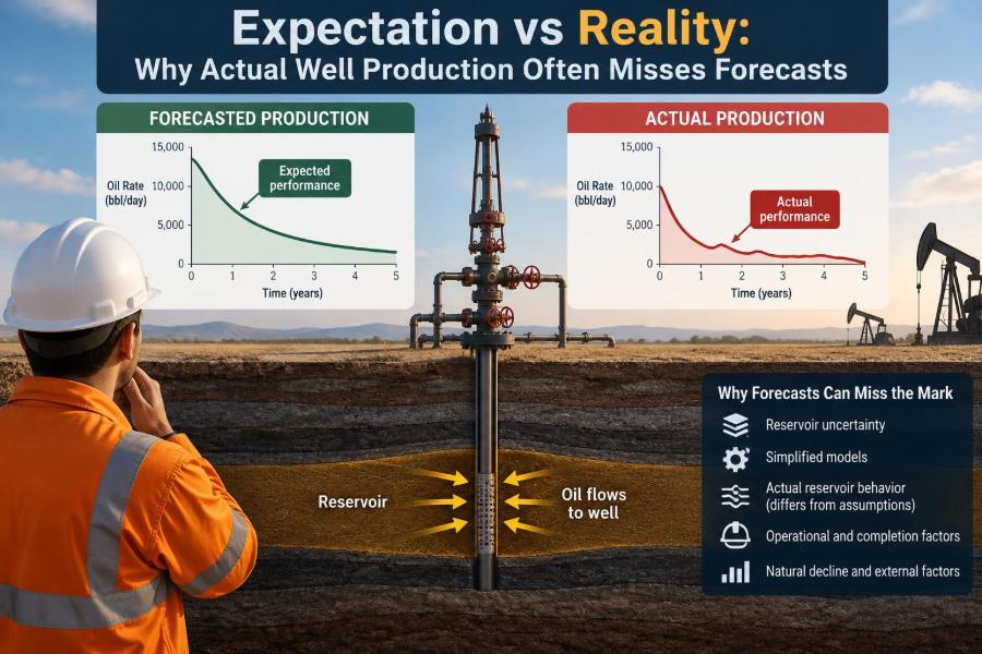

A well comes online, the first test is circulated, and the production rate is lower than the forecast in the reserves report. Or it starts strongly, only to decline much faster than expected. For engineers, managers, investors, and field teams, that gap can quickly become the most discussed number in the room.
It is tempting to treat a missed forecast as evidence that someone made a bad calculation. Sometimes there is a clear technical error. More often, however, a production forecast is a conditional estimate built from incomplete subsurface information, operational assumptions, and economic constraints that can all change after the well is drilled.
Forecasts remain essential. They guide development planning, facilities sizing, reserves evaluation, budgets, and decisions about when to drill the next well. The goal is not to eliminate uncertainty; it is to understand where it enters the forecast and manage it honestly.
The difference between expectation and reality is usually a chain of small mismatches rather than one dramatic failure. Learning to trace that chain is a core petroleum-engineering skill.
🎯 What a Production Forecast Actually Represents
A production forecast estimates future oil, gas, water, and sometimes condensate rates over time. It may describe a single well, a pad, a reservoir sector, or an entire field.
Crucially, a forecast is not a promise of future performance. It is the output of assumptions about reservoir quality, fluids, well design, completion effectiveness, operating uptime, pressure support, and commercial limits. If any assumption changes, the expected profile should change too.
🧩 Why Forecasts Begin With an Incomplete Picture
Before drilling, engineers infer the reservoir from seismic interpretation, offset wells, logs, cores, pressure data, and analog fields. Each source is valuable, but none provides a complete, continuous image of rock and fluid properties between wells.
A map can identify a promising structure while still missing a thin baffle, a fault compartment, or a local low-permeability streak. The well later samples a tiny portion of a large reservoir, so early production can reveal conditions the pre-drill model could only estimate.
🪨 Rock Quality Is Rarely Uniform
Porosity measures storage space, while permeability measures how easily fluids flow through connected pores. Two intervals with similar porosity can produce very differently if their pore throats, cementation, clay content, or natural fractures differ.
This heterogeneity is especially consequential in layered clastics, carbonates, and tight formations. A completion may contact the expected gross thickness but receive most of its flow from only a few thin, high-quality layers.
📍 A Well Is Not the Average Reservoir
Forecasts commonly use average values for permeability, net pay, saturation, and pressure. But a well does not produce from an average map cell; it produces from its exact trajectory and its immediate drainage region.
A useful analogy is a weather forecast for a city versus the weather on one street. The regional outlook may be reasonable, while a localized storm or dry pocket changes the result at a particular location.
🧭 Landing and Placement Can Change the Outcome
For horizontal wells, staying within the intended reservoir interval is often as important as reaching the planned length. Structural uncertainty, dip changes, tool limitations, and interpretation choices can place parts of the lateral closer to a boundary, water-bearing zone, or poorer rock.
Geosteering reduces this risk by updating the trajectory with real-time measurements, but it does not remove uncertainty. A lateral can be “in zone” geometrically yet still encounter poorer-than-expected reservoir quality.
🛢️ Fluid Contacts May Not Be Where the Model Put Them
Oil-water and gas-oil contacts are often represented as smooth surfaces in a model. In reality, capillary effects, tilted contacts, fault compartmentalization, and incomplete pressure communication can make fluid distributions more complex.
If a well is drilled closer to water than expected, early water production can reduce oil relative permeability and constrain drawdown. If it encounters more gas than expected, gas handling limits or changing fluid properties may alter the operating plan.
🔒 Compartments Can Shrink the Connected Volume
A fault may appear sealing, partially sealing, or transmissive depending on rock properties and pressure conditions. Small stratigraphic barriers can have similar effects. If a well accesses only one compartment, its connected hydrocarbon volume may be smaller than the mapped closure suggests.
This is one reason pressure data and interference testing are so valuable. They can indicate whether wells communicate hydraulically, although interpreting those tests also requires care.
📉 Initial Rate Is Not Ultimate Recovery
A high initial production rate can be encouraging, but it does not by itself establish a large recoverable volume. The rate may reflect high drawdown, temporary cleanup effects, near-wellbore conditions, or a limited high-permeability streak.
Conversely, a modest early rate does not automatically mean poor recovery. A well may be deliberately choked back, constrained by facilities, or producing from a reservoir that supports stable rates over a longer period.
📈 Decline Curves Need Enough History
Decline-curve analysis extrapolates production behavior from historical rates. It is widely used because it is practical, but its reliability depends on sufficient, representative production history and stable operating conditions.
Applying a decline trend too early can be misleading. A well may still be cleaning up, transitioning between flow regimes, changing choke settings, or responding to neighboring wells. Mathematical fit is not the same as physical understanding.
🧪 PVT Uncertainty Affects Rate and Volume Calculations
PVT stands for pressure-volume-temperature behavior of reservoir fluids. It governs properties such as oil formation volume factor, gas solubility, viscosity, and density, which are needed to convert surface measurements into reservoir volumes.
Representative fluid samples are not always easy to obtain. Contamination, phase changes during sampling, and limited spatial coverage can introduce uncertainty, particularly in volatile oil and gas-condensate systems.
🌡️ Pressure Depletion Changes the Production System
As reservoir pressure falls, fluid mobility and well deliverability may change. Oil below bubble-point pressure can release solution gas; gas-condensate reservoirs can experience liquid dropout near the wellbore; waterflooded reservoirs develop different pressure and saturation patterns.
A forecast must therefore represent pressure behavior, not merely start from an initial pressure. An incorrect pressure-support assumption can distort both rates and recovery timing.
💧 Water Is Both a Reservoir Signal and an Operating Challenge
Water production can arise from an aquifer, injected-water breakthrough, coning, channeling behind pipe, or completion communication with a water-bearing interval. These mechanisms require different responses, so treating all water as the same problem is a mistake.
High water cut can reduce oil throughput, increase lifting and disposal costs, and consume facility capacity. A forecast that assumes a delayed or gradual water increase may miss reality when a conductive pathway accelerates breakthrough.
🧱 Completion Quality Controls Access to the Reservoir
The reservoir may contain hydrocarbons, but the well must still connect to them effectively. Perforation depth, shot density, perforation phasing, stimulation placement, cement quality, and sand-control performance influence that connection.
Completion inefficiency can make a good reservoir look poor. Diagnostic work should separate reservoir limitation from wellbore or completion limitation before revising the geological model.
⚡ Stimulation Does Not Create a Uniform Result
Hydraulic fracturing is designed to increase conductive flow paths, but fracture geometry and conductivity are uncertain. Stress contrasts, natural fractures, fluid loss, proppant transport, and stage isolation can all alter the stimulated reservoir volume.
In a hypothetical tight-oil well, two adjacent stages may receive similar pumping schedules yet contribute very different amounts of production because one intersects better rock or a natural-fracture network. Pumping data alone cannot prove equal subsurface effectiveness.
🧯 Near-Wellbore Damage Can Hide Reservoir Potential
Drilling mud invasion, fines migration, scale, wax, emulsions, and completion debris can reduce permeability near the wellbore. This additional resistance is often described as skin.
Positive skin lowers productivity, while stimulation may reduce it. A poor early test should prompt questions about cleanup and damage before concluding that the reservoir itself lacks deliverability.
🧰 Artificial Lift Introduces Its Own Forecast Risk
Many wells require gas lift, electrical submersible pumps, rod pumps, or other lift methods as reservoir energy declines. Each system has an operating envelope and can become the rate-limiting component.
Pump wear, gas interference, insufficient power, scale, changing fluid level, and suboptimal design can create production losses not captured in a reservoir-only forecast. Production forecasting must include the whole well system.
🏭 Surface Constraints Can Cap a Technically Productive Well
A well may be capable of producing more than the facility can process. Limits can come from separator capacity, gas compression, water handling, export pipelines, flare restrictions, chemical availability, or tank logistics.
Reported production is therefore sometimes an allocated or constrained rate, not the well’s unconstrained potential. This distinction matters when calibrating a model from field data.
🔧 Downtime Is Part of Real Production
Forecasts may use an uptime assumption: the proportion of time a well is expected to be available to produce. Actual uptime is affected by planned maintenance, power interruptions, equipment failures, workovers, weather, and shared-facility outages.
Ignoring downtime produces an optimistic sales forecast even if the reservoir model is perfect. Separating “technical potential” from “expected delivered production” makes planning more transparent.
👥 Offset Wells Are Evidence, Not Copy-and-Paste Templates
Offset performance provides crucial calibration, but neighboring wells are not interchangeable. They may differ in landing depth, completion design, drawdown strategy, fluid contacts, depletion history, and local rock quality.
Analog comparisons are strongest when engineers explain why the wells are comparable. Selecting only high-performing offsets creates an optimistic bias; selecting only poor ones can be equally misleading.
🔄 Well Interference Alters Parent and Child Performance
In infill development, a new “child” well can interact with older “parent” wells through pressure depletion or hydraulic communication. The result can be accelerated decline, changed fluid distribution, or reduced stimulation effectiveness.
Spacing assumptions should therefore be tested against pressure, production, completion timing, and geological continuity. A type curve based on isolated early wells may overstate performance in a dense development program.
📊 Type Curves Can Conceal Too Much Variation
A type curve is a representative production profile, often normalized by lateral length or another scaling variable. It is useful for portfolio-level planning, but averaging can conceal a wide spread of individual results.
| Forecast input | What can differ in reality | Likely consequence |
|---|---|---|
| Average rock quality | Local sweet spot or poor-quality interval | Rate and recovery shift |
| Planned completion response | Uneven stage contribution | Different early decline behavior |
| Assumed uptime | Lift or facility downtime | Lower delivered volumes |
| Uniform spacing effect | Variable interference | Parent-child performance changes |
Good type curves show their basis, range, normalization method, and applicable operating conditions. A single “representative” line should not be mistaken for a confidence range.
🧮 Deterministic Forecasts Need Uncertainty Ranges
A deterministic case gives one answer, often called a base case. It is convenient for communication, but it can falsely imply precision when input uncertainty is large.
Scenario ranges such as low, central, and high cases expose the assumptions driving the spread. Probabilistic workflows can go further by sampling uncertain inputs, but their output is only as credible as the geological and operational assumptions behind it.
🗺️ History Matching Is Calibration, Not Proof
History matching adjusts a reservoir model so simulated pressure and production resemble observed data. It is a powerful learning tool, yet multiple combinations of permeability, boundaries, relative permeability, and aquifer strength can match the same history.
A matched model should be judged by whether its parameters remain geologically plausible and whether it predicts withheld observations. Matching every historical data point with unrealistic adjustments creates false confidence.
🧾 Measurement and Allocation Errors Matter
Production data may come from test separators, multiphase meters, tank measurements, allocation calculations, or periodic well tests. Each method has limitations, particularly when flow is unstable or water and gas fractions change quickly.
Before diagnosing a reservoir problem, verify the data chain: meter calibration, test duration, allocation method, shut-in records, choke history, and unit conversions. A flawed rate history can mislead every downstream interpretation.
🔍 Production Surveillance Turns Surprises Into Knowledge
Surveillance includes pressure measurements, fluid sampling, production logging, tracers, temperature data, well tests, and routine operating records. The appropriate tool depends on the question being asked.
For example, production logging may help locate water entry, while pressure surveillance can reveal depletion or compartment behavior. The best program is focused: collect data that can change a decision, not data simply because it is available.
🛠️ Diagnose Before Choosing a Fix
When production misses forecast, common reactions include increasing drawdown, stimulating again, adding lift, shutting off water, or drilling another well. Any of these may be appropriate, but each can be costly or harmful if the diagnosis is wrong.
- Check whether the reported rate is constrained by facilities or downtime.
- Review well integrity, completion records, and artificial-lift performance.
- Compare pressure and fluid behavior with the reservoir model.
- Identify whether the issue is local, area-wide, or related to interference.
- Update the forecast only after documenting the evidence and remaining uncertainty.
⚖️ Avoid Blaming Either the Reservoir or Operations Too Quickly
Reservoir teams may attribute underperformance to poor rock, while operations teams may focus on mechanical restrictions. Both explanations can be partly true, and separating them requires collaboration.
An integrated review combines geology, petrophysics, reservoir engineering, production engineering, completions, facilities, and commercial context. The question is not “who owns the miss?” but “what mechanism best explains the data?”
🧠 Forecast Assumptions Should Be Visible and Testable
A useful forecast records the assumptions behind it: drainage area, net pay, pressure support, well spacing, completion efficiency, decline behavior, uptime, facility limits, and abandonment criteria. Hidden assumptions are difficult to challenge and impossible to learn from systematically.
For each major assumption, define an observable trigger. If water cut rises earlier than expected, if pressure declines faster, or if uptime falls, the team should know which forecast element needs review.
📅 Update Forecasts at Decision Points
Constantly changing a forecast can create noise, while refusing to update it preserves an outdated story. The practical balance is to revise forecasts when new data materially affect decisions such as drilling sequence, facility expansion, reserves booking, or intervention timing.
Early-life updates may be frequent because uncertainty is resolving quickly. Later updates can focus on meaningful shifts in decline, water handling, pressure behavior, and operating reliability.
🧑🏫 What Students and Early-Career Engineers Should Practice
Learn to ask what physical mechanism sits behind every curve. A spreadsheet can calculate a decline, but engineering judgment asks whether the observed trend is stable, constrained, or distorted by changing operations.
Practice building simple sensitivities before complex models: vary permeability, connected volume, skin, water breakthrough timing, uptime, and drawdown. This reveals which uncertainties deserve better data and which have little practical effect.
🤝 Communicating a Miss Without Losing Credibility
Clear communication distinguishes observed facts from interpretations. Say what changed, what evidence supports the proposed mechanism, what remains uncertain, and what action is recommended.
Do not hide a miss behind vague language, but do not overstate a preliminary diagnosis either. Decision-makers need the range of credible outcomes and the conditions that would move the case toward each end of that range.
🏁 The Core Principle: Forecasts Are Living Engineering Hypotheses
Actual well production misses forecasts because reservoirs are variable, wells are imperfect connections to those reservoirs, and real operations introduce constraints that models simplify. A forecast becomes more valuable when it states these limits rather than pretending they do not exist.
The strongest teams treat variance as information. They preserve the original assumptions, compare them with surveillance data, identify the most likely mechanisms, and feed the lessons into the next location, completion, facility plan, and forecast.
A credible production forecast is not the one that looks most certain; it is the one that makes uncertainty visible, testable, and useful for better decisions. 🛢️📈🔍