
A drilling team reaches a formation at 10,000 ft true vertical depth and needs to decide whether the mud weight provides enough bottomhole pressure. A reservoir engineer is reviewing an initial pressure test and wants to know whether its measured gradient is consistent with oil, water, or gas. In both cases, the starting point is hydrostatic pressure.
The calculation looks simple: fluid density multiplied by gravity and vertical height. Yet small mistakes with units, depth reference, or density basis can produce a pressure estimate that is misleading enough to affect well control, completion design, or reserve interpretation.
Hydrostatic pressure is not a prediction of every pressure a well will encounter. It is the pressure created by a fluid column at rest. Real reservoirs can be depleted, overpressured, compartmentalized, or connected to aquifers, so the calculation must be used with geological and operational context.
Still, learning to calculate it correctly gives petroleum engineers a powerful reference line. It helps turn density and depth into a physically meaningful pressure estimate.
🧭 1. What Reservoir Hydrostatic Pressure Means
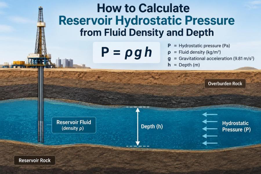
Reservoir hydrostatic pressure is the pressure exerted by the weight of reservoir fluid above a chosen point when that fluid is static. The deeper the point, the larger the fluid column and the higher its pressure.
Imagine standing at the bottom of a swimming pool: water pressure is greater there than at the surface because more water sits above you. Reservoir fluids behave by the same fundamental principle, although their density, compressibility, temperature, and phase behavior are more complicated.
Pressure is normally reported at a stated depth and relative to a specified datum. Without both pieces of information, a pressure value is incomplete.
📐 2. The Fundamental Equation
The basic hydrostatic relation is:
ΔP = ρgΔzHere, ΔP is the pressure change, ρ is fluid density, g is gravitational acceleration, and Δz is the vertical depth difference. The equation calculates a pressure difference, not automatically an absolute reservoir pressure.
To calculate pressure at depth from a reference point, add the pressure at that reference:
P₂ = P₁ + ρg(z₂ - z₁)This form makes the required reference explicit. If depth increases downward, the pressure at the deeper point increases for a normal fluid column.
⚖️ 3. Why Density Controls the Gradient
A denser fluid weighs more per unit volume, so it creates a steeper pressure increase with depth. Brine generally has a higher hydrostatic gradient than oil, while gas usually has a much lower and less constant gradient.
Density is not merely a laboratory property. Reservoir-fluid density varies with pressure, temperature, dissolved gas, salinity, and composition. A calculation is only as representative as the density selected for it.
For a short vertical interval, using one average density is often reasonable. Across a tall hydrocarbon column or a deep gas reservoir, density variation may need explicit treatment.
📏 4. Use True Vertical Depth, Not Measured Depth
Hydrostatic pressure depends on vertical height, so use true vertical depth (TVD), or a vertical depth difference between points. Measured depth (MD) follows the wellbore path and becomes much longer than TVD in deviated and horizontal wells.
A horizontal section may add thousands of feet of MD with almost no additional hydrostatic head. Substituting MD for TVD would incorrectly imply a large pressure increase simply because the wellbore curves.
Check the depth convention carefully: TVD, TVD subsea (TVDSS), and depth below rotary table are not interchangeable unless their datum offsets are accounted for.
🌊 5. Choose a Clear Pressure Datum
Every pressure calculation needs a reference pressure and reference elevation. Common datums include mean sea level, a fluid contact, a perforation depth, a pressure gauge depth, or a defined reservoir datum.
For example, if a water pressure is known at 8,000 ft TVDSS, calculate the expected pressure at 8,500 ft TVDSS by applying the water gradient across 500 ft. Do not silently mix a subsea depth with a depth referenced to the rig floor.
A good pressure report states pressure, depth, vertical datum, fluid assumed, and the units used.
🔢 6. Work in Consistent SI Units
In SI units, use density in kilograms per cubic metre, gravity in metres per second squared, and vertical depth in metres. The result from ρgΔz is pascals.
ΔP (Pa) = ρ (kg/m³) × 9.80665 (m/s²) × Δz (m)Engineers commonly convert pascals to megapascals: 1 MPa = 1,000,000 Pa. A fluid with density 1,000 kg/m³ creates approximately 9.81 MPa per 1,000 m of vertical depth.
Using 9.81 m/s² is normally sufficient for engineering calculations unless a project requires a more specific gravity convention.
🛢️ 7. Use Oilfield-Unit Shortcuts Carefully
In field units, hydrostatic pressure is often estimated from fluid density in pounds per gallon (ppg) and depth in feet:
ΔP (psi) ≈ 0.052 × density (ppg) × ΔTVD (ft)The factor 0.052 incorporates unit conversions and standard gravity. It is widely used for drilling fluids and provides a convenient check on bottomhole pressure calculations.
Another useful form uses a pressure gradient directly:
ΔP (psi) = gradient (psi/ft) × ΔTVD (ft)Use the shortcut only when density, depth, and pressure units match the equation. A factor memorized for ppg and feet cannot be transferred to kilograms per cubic metre and metres.
🧪 8. Convert Specific Gravity to Density
Specific gravity (SG) is the ratio of a fluid’s density to the density of water at a stated reference condition. It has no units. For a first-pass calculation, density can be estimated as:
ρfluid ≈ SG × 1,000 kg/m³For example, a liquid with SG 0.85 has an approximate density of 850 kg/m³. Its pressure gradient is lower than freshwater’s because each metre of fluid weighs less.
Be precise when the calculation supports a formal decision. The density of water itself changes with salinity, temperature, and pressure, so a reference-density assumption should be documented.
💧 9. Estimate the Water Gradient
Freshwater near surface conditions has a gradient of about 0.433 psi/ft, or about 9.81 kPa/m. Formation water is often saline and can be denser, producing a larger gradient.
Suppose a brine density is 1,080 kg/m³. Its approximate SI gradient is:
1,080 × 9.81 = 10,595 Pa/m ≈ 10.60 kPa/mAcross 500 m of vertical brine column, the hydrostatic pressure increase is approximately 5.30 MPa. This is a pressure difference across that interval, not the total pressure unless the reference pressure is included.
🟤 10. Estimate the Oil Gradient
Oil density is usually lower than water density, so oil has a smaller pressure gradient. A hypothetical oil density of 800 kg/m³ gives:
800 × 9.81 = 7,848 Pa/m ≈ 7.85 kPa/mAcross 1,000 m TVD, that oil column contributes roughly 7.85 MPa of pressure difference. In field-unit terms, an oil gradient may be around a few tenths of a psi per foot, depending on oil density.
Live oil density at reservoir conditions can differ substantially from stock-tank oil density. Use pressure-volume-temperature (PVT) data when available rather than treating a surface density as automatically representative.
💨 11. Treat Gas Columns Differently
Gas is highly compressible. Its density changes significantly with pressure and temperature, so a single constant-density calculation may be suitable only for a rough, short-interval estimate.
For a gas column over a meaningful vertical range, calculate density as a function of pressure and temperature, then integrate the pressure gradient numerically. An equation of state or validated PVT model is commonly needed.
The key practical consequence is that pressure-versus-depth for gas is generally curved, while a liquid with nearly constant density produces an approximately straight line.
📈 12. Read Pressure Gradient Plots
A pressure-depth plot is one of the clearest ways to interpret hydrostatic behavior. Plot pressure on the horizontal axis and TVDSS on the vertical axis, with depth increasing downward by convention.
For a liquid of nearly constant density, data points should align along a straight line. The slope represents the pressure gradient. A steeper slope indicates a denser fluid.
Separate straight lines may identify oil and water zones. Their intersection can help constrain a fluid contact, provided the measurements are reliable and the fluids are in pressure communication.
🧱 13. Calculate Across a Single Fluid Column
When the reservoir interval contains one fluid and density is approximately constant, the workflow is direct:
- Define the reference pressure and its vertical depth.
- Identify the pressure-point depth in the same datum.
- Find the vertical depth difference.
- Apply the appropriate fluid density or pressure gradient.
- Add or subtract the resulting pressure difference according to the depth direction.
Keeping the calculation as a sequence prevents a common error: applying a gradient to total depth when the known pressure already belongs to a deeper or shallower reference point.
🌗 14. Handle Oil-Water Columns in Segments
A reservoir with an oil-water contact contains fluids with different gradients. The pressure change from a reference point to a target depth must be calculated in separate segments.
For a target below the contact, first move from the reference point through the oil column to the contact using the oil gradient. Then move through the water column from the contact to the target using the water gradient.
This segmented method matters because replacing both fluids with one average gradient can distort predicted pressures and obscure the physical meaning of the contact.
🧮 15. A Worked Oil-Water Example
Consider a hypothetical reservoir where pressure at 2,000 m TVDSS is 20.0 MPa in an oil zone. The oil-water contact is at 2,200 m TVDSS. Oil density is 800 kg/m³, and brine density is 1,080 kg/m³. Estimate pressure at 2,500 m TVDSS.
From 2,000 to 2,200 m, the oil pressure increase is approximately 800 × 9.81 × 200 = 1.57 MPa. Pressure at the contact is therefore about 21.57 MPa.
From 2,200 to 2,500 m, brine adds approximately 1,080 × 9.81 × 300 = 3.18 MPa. The estimated pressure at 2,500 m is 24.75 MPa, subject to the constant-density assumptions.
🧷 16. Distinguish Gauge and Absolute Pressure
Absolute pressure is measured relative to a vacuum. Gauge pressure is measured relative to local atmospheric pressure. Reservoir engineering data are commonly reported as absolute pressure, but field instruments and operational discussions can vary.
The hydrostatic pressure difference is the same regardless of whether the starting pressure is gauge or absolute. Trouble arises when a gauge reference is added to an absolute measurement without converting one basis to the other.
Label pressure units clearly, such as psia versus psig, or MPa absolute versus MPa gauge, especially when transferring data between operations and subsurface teams.
🌡️ 17. Account for Temperature Effects
Temperature changes fluid density. Liquids usually expand and become less dense as temperature rises, although the exact response depends on composition and pressure. Reservoir fluids at depth may therefore not share surface densities.
For screening calculations, a representative reservoir-condition density may be enough. For fluid contacts, pressure matching, or narrow operating margins, use density values from a relevant PVT study or a calibrated fluid model.
Temperature also varies vertically in most basins. That variation is another reason a single density can become less reliable over a long column.
🗜️ 18. Recognize Pressure Effects on Density
Liquids are often treated as incompressible, but they are not perfectly so. At high pressure, their density changes enough that a constant-density approximation may introduce a noticeable cumulative error over large depth ranges.
Gas demands more care because compressibility is central to its behavior. As pressure increases downward, gas generally becomes denser, increasing its local hydrostatic gradient.
A practical rule is to match model complexity to the decision. A hand estimate can screen possibilities; a development plan or close pressure-contact interpretation deserves a PVT-consistent calculation.
🧭 19. Separate Hydrostatic Pressure from Reservoir Pressure
Hydrostatic pressure describes the expected pressure variation within a static, connected fluid column. Reservoir pressure is the actual pressure measured or inferred at a particular location and time.
A reservoir can be underpressured after production, overpressured because of geological processes, or locally isolated by faults and low-permeability barriers. In such cases, hydrostatic gradients still describe fluid-column behavior, but the reference pressure may differ from a simple regional expectation.
Do not assume that a depth alone determines reservoir pressure. It determines the hydrostatic contribution once the correct fluid system and reference condition are known.
⚠️ 20. Investigate Deviations from a Hydrostatic Trend
When pressure data do not fall on the expected gradient, do not immediately conclude that the data are wrong. The deviation may reveal useful subsurface information.
- Different fluid types or changing fluid composition
- Separate pressure compartments across sealing faults
- Production-related depletion near one well
- Supercharging or transient pressure-tool effects
- Incorrect depth conversion or datum mismatch
- Poor pressure-test quality or insufficient buildup time
Interpretation should combine pressure data with logs, fluid samples, completion history, structural maps, and test conditions.
🛠️ 21. Apply the Calculation to Drilling Fluids
During drilling, mud density creates hydrostatic bottomhole pressure. The familiar field estimate is:
Hydrostatic pressure (psi) ≈ 0.052 × mud weight (ppg) × TVD (ft)This static estimate is essential, but circulating conditions add frictional pressure losses. The resulting equivalent circulating density can exceed the static mud density effect at the bottomhole.
For well-control and narrow-margin drilling decisions, include annular friction, surge and swab effects, temperature, cuttings loading, and pressure uncertainty. A static hydrostatic calculation is the foundation, not the complete hydraulics model.
🧰 22. Use a Reproducible Calculation Template
A clear calculation sheet or spreadsheet should make review easy. Record the inputs before entering the formula:
- Pressure reference value and whether it is absolute or gauge
- Reference depth and target depth, with the vertical datum
- Fluid identity and density basis
- Gravity convention and unit system
- Assumptions, including constant density or segmented fluids
- Calculated pressure difference and final target pressure
This documentation is especially valuable when several disciplines use the result. It lets another engineer reproduce the answer and identify whether a difference comes from geology, fluid properties, or units.
❌ 23. Avoid Common Calculation Mistakes
The most frequent error is mixing units: metres with a psi-per-foot gradient, kilograms per cubic metre with a field-unit conversion factor, or MPa with kPa. Dimensional checks catch many of these mistakes before they reach a report.
Other recurring problems include using MD rather than TVD, applying a surface density to deep live oil, ignoring an oil-water contact, and omitting the reference pressure. Each can produce an answer that looks numerically tidy but has the wrong physical basis.
Also avoid excessive precision. Reporting many decimal places from uncertain density, depth, or contact inputs suggests accuracy that the data do not support.
✅ 24. Perform Quick Quality Checks
Before accepting a result, ask whether the sign makes sense: pressure should increase when moving downward through a normal static fluid column. Then compare the implied gradient with the fluid type. Water should generally be steeper than oil, and gas should not be treated as a constant-density liquid without justification.
Check the magnitude against a simple mental estimate. A water-like liquid adds roughly 10 MPa per kilometre of vertical depth. If a result differs dramatically, revisit units, depth, and density.
Finally, compare calculated values with measured formation-pressure data where available. Agreement supports the assumptions; disagreement is a prompt to investigate, not an invitation to force the numbers to match.
🧠 25. The Core Principle to Carry Forward
Hydrostatic pressure calculation begins with a simple physical idea: a deeper point supports more fluid weight above it. In practice, reliable work depends on four disciplined choices: use vertical depth, establish a common datum, select reservoir-condition fluid density, and keep units consistent.
Use ΔP = ρgΔz for a constant-density fluid interval, divide mixed columns into their individual fluid segments, and use a variable-density approach when gas or large pressure-temperature changes make it necessary. The calculation provides a reference framework for interpreting actual reservoir pressures, not a substitute for measurements and geological understanding.
Calculate the fluid weight correctly, state the assumptions openly, and let measured pressure data test the hydrostatic model. That habit turns a basic equation into a dependable engineering tool. 🛢️📐