
A producing well can look healthy on a daily report and still be moving toward a difficult economic decision. Its rate may be lower than last month, water handling may be increasing, or a planned workover may no longer appear attractive. The question is not simply, “What did the well produce?” It is, “What is it likely to produce next?”
That question influences reserve estimates, facility sizing, artificial-lift planning, field budgets, and the timing of abandonment. It also matters to engineers trying to explain a reservoir’s behavior without waiting years for every uncertainty to disappear.
Decline curve analysis offers a practical way to turn production history into a forward-looking forecast. It is widely used because rate and time data are available for most producing wells, even when subsurface data are incomplete.
But a decline curve is not a crystal ball. Used thoughtfully, it reveals production trends and exposes questions worth investigating. Used mechanically, it can disguise operational interruptions, changing constraints, or reservoir behavior that the chosen curve cannot represent.
🛢️ Decline Curves in Plain Language
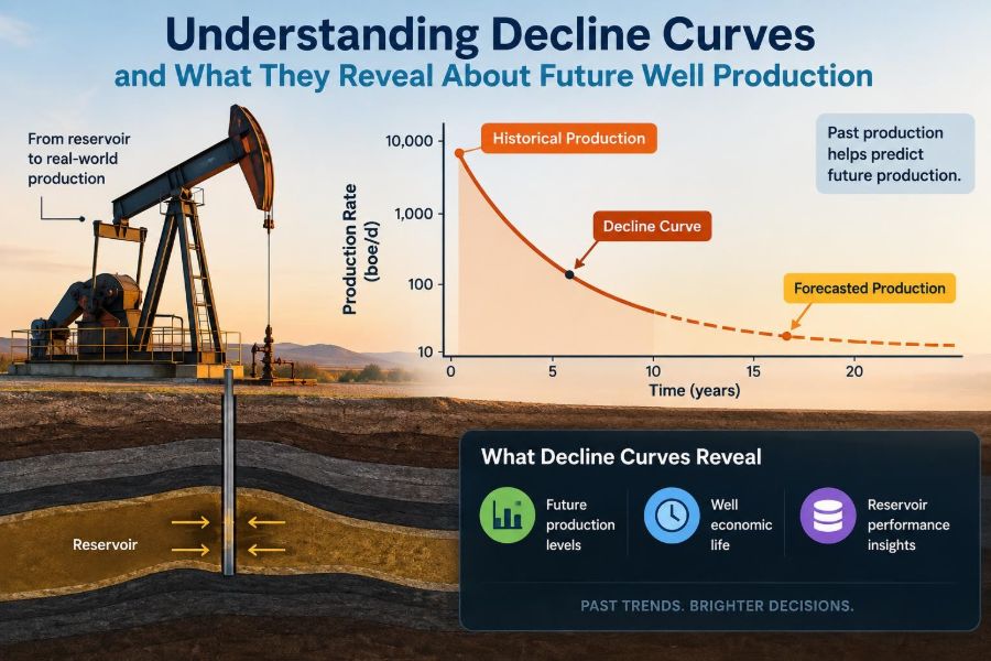
A decline curve is a mathematical description of how a well’s production rate falls with time or cumulative production. The analyst fits a trend to historical oil, gas, or fluid rates and projects that trend into the future.
The basic idea is familiar outside petroleum engineering. A new phone battery may lose charge quickly at first and more gradually later. Likewise, many wells produce rapidly after startup, then decline as pressure, flowing conditions, and accessible fluid volumes change.
A decline forecast usually produces three useful outputs: future rate, future cumulative production, and estimated ultimate recovery (EUR). Each output depends on the assumptions embedded in the trend.
📉 Why Production Declines at All
Hydrocarbons flow only when there is enough energy to move them from the reservoir to the wellbore and then to surface facilities. That energy may come from natural reservoir pressure, gas expansion, water influx, gravity drainage, or artificial lift.
As fluids are withdrawn, pressure near the well commonly falls. The pressure difference driving flow can shrink, and the path to the well may become less favorable as relative permeability changes, gas evolves from solution, or water saturation increases.
Surface conditions also matter. Higher flowing wellhead pressure, a restricted choke, degrading lift equipment, or limited facility capacity can reduce observed production even if the reservoir itself has not changed in the same way.
🧭 What a Forecast Actually Reveals
A projected decline is best understood as a conditional statement: if the well continues operating under comparable reservoir and operating conditions, its future production may follow this range of behavior. The condition is as important as the projected number.
For a mature conventional well with stable operations, the curve may provide a useful description of depletion. For a recently stimulated horizontal well, it may instead summarize an early transient flow period that has not yet settled into longer-term behavior.
The curve therefore reveals both a production expectation and the sensitivity of that expectation to assumptions. A long economic tail can add significant cumulative volume, but it is often the least certain portion of a forecast.
🗂️ The Production Data Behind the Curve
Good decline analysis begins with production allocation and measurement, not curve fitting. Common inputs include oil, gas, water, condensate, operating time, well status, flowing pressures, choke settings, and artificial-lift records.
Monthly data are common for reserves work because they reduce daily noise and match many reporting systems. Daily data can be valuable for diagnosing operations, but they may make a long-term trend look more erratic than it is.
Before interpreting a rate, ask whether it represents a full producing period. A monthly volume divided by calendar days can look like a reservoir decline when the well was actually shut in for repairs.
🧹 Data Cleaning Is Engineering, Not Cosmetics
Raw production history often contains missing readings, estimated allocations, test volumes, negative adjustments, and changes in reporting conventions. Removing or correcting data without documenting the reason can create a tidy but misleading forecast.
Useful screening checks include:
- Confirming that reported volumes and operating hours are physically plausible.
- Separating shut-ins, curtailments, start-ups, and post-workover periods.
- Checking whether a meter, separator, allocation method, or ownership interest changed.
- Comparing sudden rate shifts with pressure, choke, lift, and intervention records.
A point that looks like an outlier may be a data error, but it may also be the first evidence of water breakthrough, scale deposition, or equipment failure. The goal is to explain the point before excluding it.
⏱️ Calendar Time Versus Producing Time
Calendar-time decline uses elapsed time, including downtime. It is often appropriate for business planning because revenue and facility loading are affected by real operating availability.
Producing-time decline adjusts the timeline or rate for active production time. It can better isolate reservoir performance when downtime is unrelated to depletion, such as a temporary pipeline outage.
Neither view is universally correct. A forecast should state which basis it uses and why. Confusing the two can overstate decline during frequent downtime or overstate deliverability by assuming perfect future uptime.
📐 The Arps Family of Decline Models
The most familiar production-decline equations are associated with J. J. Arps. They describe a decline rate that changes according to an exponent, commonly called b, and are often applied after a well enters boundary-dominated flow.
In practical terms, the Arps family includes exponential, harmonic, and hyperbolic decline. These are not labels to select by appearance alone; each implies a different future rate behavior and cumulative recovery.
The governing form is commonly written as q(t) = qi / (1 + b Di t)^(1/b), where q is rate, qi is an initial reference rate, Di is nominal initial decline, and b shapes how decline changes over time.
📏 Exponential Decline and Constant Percentage Loss
With exponential decline, the percentage rate loss per equal time interval remains constant. The curve becomes a straight line on a semilog plot of rate versus time, which makes it easy to recognize and communicate.
Exponential behavior is often a reasonable late-life approximation for many mature wells or for a stabilized portion of a field. It is also conservative relative to an unconstrained high-b hyperbolic tail.
Its limitation is that it may not capture a well whose decline is still flattening. Forcing early, rapidly changing production into exponential decline can underestimate near-term performance or create an unrealistic transition.
〰️ Harmonic Decline and Its Long Tail
Harmonic decline is the special Arps case where b = 1. The decline rate decreases substantially with time, producing a long tail of low-rate production.
That long tail can generate large calculated cumulative volumes if the forecast is extended indefinitely. In real operations, however, wells stop producing when they reach an economic, mechanical, contractual, or facility limit.
Harmonic decline should therefore be paired with a credible terminal condition. A mathematically valid curve is not automatically an economically recoverable forecast.
📈 Hyperbolic Decline and the b-Factor
Hyperbolic decline falls rapidly at first and then progressively flattens. Its b-factor lies between the exponential and harmonic cases in the traditional Arps framework, although fitted values can exceed one when analysts apply the equation to transient unconventional-well data.
A higher b-factor generally creates a flatter late-time tail and a larger EUR. Small changes in b can have modest effects near term but very large effects many years later.
This sensitivity is why the b-factor should not be treated as a convenient curve-shaping control. It needs support from analog wells, flow-regime understanding, and a defensible terminal-decline policy.
🔄 Nominal Decline and Effective Decline
Decline terminology causes avoidable mistakes. Nominal decline is the continuous parameter used in many equations, while effective decline is the actual fractional change over a stated period, such as a year.
For exponential decline, a nominal annual decline of D corresponds to an annual effective decline of 1 - e^(-D). The two values are related but not numerically identical.
Reports should state the convention and time basis. A forecast can appear inconsistent simply because one team is discussing nominal decline and another is comparing annual effective decline.
🧮 Rate-Time Plots and Diagnostic Shape
A rate-time plot is often the starting diagnostic. Plotting monthly oil or gas rate against time can show startup effects, step changes, downtime, and whether the decline is visibly flattening.
A semilog plot is especially helpful for exponential behavior, while a log-log plot may help reveal changing flow regimes. No single plot proves a reservoir mechanism, but multiple views prevent analysts from trusting a visually convenient line.
Plotting water rate and gas-oil ratio beside hydrocarbon rate can be revealing. A falling oil rate accompanied by rapidly increasing water is a different problem from a similarly falling oil rate with stable water production.
📊 Rate-Cumulative Plots as a Second Lens
Rate versus cumulative production, often called a q–Np plot for oil, can reduce the direct influence of time and focus attention on depletion. In some settings, a linear or smoothly changing relationship can provide a useful alternative forecast view.
It is particularly valuable when calendar time contains irregular interruptions. If the relationship changes sharply after a workover, compression project, or water breakthrough, the plot may make that discontinuity easier to see.
Rate-cumulative methods still require judgment. They do not remove uncertainty about future operating conditions or guarantee that the observed relationship will continue.
🛑 Separating Reservoir Decline From Downtime
Imagine a hypothetical well producing steadily until an electric submersible pump fails. Its reported monthly rate collapses, then rebounds after replacement. Fitting one curve through the collapse would manufacture a reservoir decline that never occurred.
Events worth flagging include pump failures, rod-parting repairs, compressor outages, line pressure restrictions, power curtailments, paraffin treatment, and planned shut-ins. Production may need to be normalized, segmented, or modeled with downtime explicitly included.
Downtime itself remains commercially relevant. The key is to avoid calling an operational availability problem a reservoir-performance problem.
🔧 The Effect of Workovers and Interventions
Acidizing, refracturing, perforating additional intervals, changing artificial lift, and removing skin can alter a well’s productive capacity. A post-intervention rate may not belong on the same uninterrupted trend as pre-intervention history.
Sometimes the correct approach is to start a new decline segment after the intervention. In other cases, the intervention restores the previous trend after a temporary impairment. The decision should rely on engineering evidence, not just the desire for a higher forecast.
Intervention forecasts should distinguish base decline from incremental response. This makes it clearer which volumes are expected from natural continuation and which depend on successful execution.
🧪 Flow Regimes Explain Why Early Curves Mislead
New wells do not necessarily decline under boundary-dominated conditions. Early production can be governed by transient flow, cleanup, fracture-fluid recovery, changing choke strategy, or interference that has not yet developed.
In unconventional reservoirs, a long transient period can make classical Arps extrapolation especially uncertain. A high early b-factor may describe observed history well while implying a late-life recovery that is difficult to justify physically.
Modern workflows may combine decline analysis with rate-transient analysis, pressure data, reservoir simulation, or calibrated analogs. The appropriate tool depends on data quality, well maturity, and the decision at stake.
🪨 Reservoir Quality and Depletion Behavior
Permeability, porosity, thickness, fluid properties, compartmentalization, natural fractures, and drive mechanism all influence decline. Two wells with similar initial rates can have very different futures because their drainage volumes and flow pathways differ.
A well in a connected, pressure-supported reservoir may decline more gradually than an isolated well with limited connected volume. Conversely, strong water influx can sustain total fluid rate while reducing oil rate and increasing water-handling costs.
Decline analysis is strongest when it is interpreted alongside geology and reservoir understanding. A curve should be asked to agree with the subsurface story, not replace it.
💧 Water Production Changes the Economic Story
Oil rate alone does not determine a well’s future value. As water cut rises, lifting, treating, transporting, and disposing of water can consume capacity and increase operating expense.
A well can continue producing measurable oil while approaching its economic limit: the point where expected revenue no longer justifies operating costs and obligations. The limit varies by field, infrastructure, fluid handling, price assumptions, and contractual conditions.
Forecasting water alongside oil is therefore essential for mature assets. A hydrocarbon decline curve without a water forecast may overstate both operating life and recoverable reserves.
🔥 Gas Wells Need Their Own Context
Gas-well analysis often requires close attention to flowing pressure and deliverability. A falling gas rate may reflect depletion, increasing backpressure from gathering systems, liquid loading, compression changes, or choke management.
Gas material balance and pressure-normalized rate methods can sometimes add insight that a simple rate-time curve misses. Condensate dropout near the wellbore may also reduce effective gas permeability and alter apparent decline behavior.
As with oil wells, a forecast based only on reported sales volume can confuse facility constraints with reservoir capacity. The measurement point and flowing conditions matter.
⚙️ Artificial Lift Can Reshape Observed Decline
Rod pumps, gas lift, electric submersible pumps, progressive cavity pumps, and plunger lift influence the drawdown a well can sustain. A change in lift method or operating setting can change rate without changing the hydrocarbon volume remaining in place.
For example, an under-pumped oil well may appear to have a steep decline until a pump optimization increases fluid rate. The apparent improvement is operational, although it may also accelerate future depletion depending on reservoir response.
Forecasts should record lift assumptions: pump capacity, gas interference, fluid level, injection-gas availability, run life, and expected optimization. Ignoring lift constraints can turn a technically possible rate into an operationally impossible one.
🏭 Facilities and Constraints Are Part of the Forecast
A well does not produce in isolation. Separator pressure, pipeline capacity, compressor availability, produced-water capacity, flare limits, and shared power systems can all control actual sales volumes.
When several wells are constrained together, individual decline curves may overstate field deliverability. A field forecast must honor the network and allocate constraints realistically.
Conversely, a debottlenecking project can create a rate uplift that should not be mistaken for a reservoir improvement. Keeping reservoir potential separate from constrained production makes planning more transparent.
🧩 Segmenting a Complex Production History
One equation across the entire life of a well is often too simple. Segmentation can be appropriate when there is a clear, explainable change in operating mode, completion, pressure support, or facility condition.
A sound segment boundary has a physical or operational reason. A weak boundary is simply placed where it improves the regression fit.
Document each segment’s start date, rationale, data treatment, and forecast rule. This allows another engineer to review the logic and avoids hidden adjustments during reserves reviews or asset handovers.
🔍 Choosing an End Point for the Forecast
Production forecasts should not run forever. Common termination criteria include an economic limit, a minimum rate, a maximum water cut, an abandonment date, lease conditions, or the end of a development-plan period.
The terminal rate should reflect actual operating economics rather than a generic value applied to every well. A low-rate well tied to existing infrastructure can remain economic longer than an isolated well requiring dedicated handling.
For some reserve classifications, additional commercial and project criteria apply beyond technical producibility. Decline analysis informs those decisions but does not independently establish them.
💼 From Decline Curves to Reserves and Value
Forecast volumes feed reserve estimates, production targets, operating budgets, and economic evaluations. Because the forecast tail can strongly affect cumulative recovery, assumptions must be visible and internally consistent.
Reserve work commonly uses scenario ranges rather than a single deterministic answer. The range should reflect material uncertainties such as well performance, downtime, water costs, commodity prices, planned interventions, and abandonment timing.
A curve fit with many decimal places is not evidence of precision. The useful question is whether its assumptions are appropriate for the decision and whether the resulting range is credible.
🎯 Building Low, Base, and High Cases
A practical forecast rarely has one “correct” curve. Low, base, and high cases can represent different but plausible outcomes, provided each case has a stated technical basis.
- Low case: earlier economic limit, weaker productivity, more downtime, or faster water-related decline.
- Base case: continuation of the most supportable operating and reservoir trend.
- High case: stronger performance, successful optimization, or a favorable but realistic analog-supported outcome.
Scenario differences should not be arbitrary percentage adjustments. Tie them to identifiable uncertainties so decision-makers understand what would need to happen for each outcome.
⚠️ Common Curve-Fitting Mistakes
Several errors recur because curve-fitting software makes it easy to generate a smooth projection:
- Fitting through shut-ins, unplanned downtime, or unreliable allocations.
- Using early transient data as though it represented stabilized depletion.
- Allowing an aggressive hyperbolic tail to continue without a terminal-decline rule.
- Ignoring water, lift, pressure, and facility constraints.
- Selecting the highest EUR because it gives the best statistical fit.
- Failing to update a forecast after new production contradicts its assumptions.
The common thread is overreliance on the equation and underuse of engineering context.
🧠 A Disciplined Decline Analysis Workflow
A repeatable workflow improves both speed and auditability. Start by defining the purpose: surveillance, budget planning, reserves, intervention screening, or facility design. The required precision and conservatism may differ.
- Assemble rates, volumes, uptime, pressures, water, gas, and event history.
- Validate measurements and identify operationally abnormal periods.
- Plot data in several diagnostic forms before selecting a model.
- Choose a decline form or segmented approach consistent with flow behavior.
- Apply operating, facility, water-handling, and economic limits.
- Compare results with analogs and reservoir expectations.
- State uncertainties, preserve assumptions, and update as new data arrive.
This sequence prevents a polished chart from becoming the starting and ending point of the analysis.
🤝 Using Analogs Without Copying Them Blindly
Analog wells can constrain forecasts where history is short. The best analogs share meaningful features: completion design, lateral length where relevant, reservoir interval, fluid type, operating strategy, pressure environment, and nearby development conditions.
A neighboring well is not automatically a good analog. It may have different landing depth, stimulation intensity, interference exposure, or artificial-lift performance.
Use analogs to test whether a forecast is plausible, not to overwrite well-specific evidence. When the subject well diverges, investigate the reason before averaging the difference away.
🗣️ Communicating Results So Others Can Use Them
An effective forecast presentation shows history, fitted segments, future cases, key events, terminal criteria, and a brief assumptions list. Readers should be able to see what is data, what is interpretation, and what is contingent on a future action.
Use clear units and label whether rates are gross or net, allocated or tested, and calendar-time or producing-time based. These distinctions can materially change comparisons between wells.
For management audiences, connect the decline to decisions: expected cash-flow timing, compression need, workover timing, water capacity, or abandonment exposure. Technical detail matters most when it changes an action.
🔁 Updating the Forecast Is a Core Practice
Every new month of production tests the prior forecast. A variance is not automatically a failure; it may reveal changing operations, better-than-expected uptime, emerging water issues, or a shift in reservoir behavior.
Track forecast-versus-actual performance by rate and cumulative volume. Then separate whether variance arose from uptime, constraints, intervention results, measurement changes, or genuine well deliverability.
Regular updates turn decline analysis into a surveillance tool rather than a one-time estimate filed away after a planning cycle.
🧭 The Core Principle: Curves Need Context
Decline curves are powerful because production history contains real information about a well’s performance. They can translate that history into practical estimates of future rate, cumulative recovery, operating life, and uncertainty.
Yet the strongest forecast is not the one with the smoothest mathematical fit. It is the one that reconciles rate data with flow regime, reservoir characteristics, pressure and lift conditions, downtime, water behavior, facilities, economics, and analog performance.
When a curve and the physical story disagree, the disagreement is valuable. It is a prompt to inspect the data, revisit assumptions, and decide whether the well has changed—or whether the analysis has.
A decline curve should be treated as an engineering hypothesis, continually tested against production reality, rather than a promise about the future. That mindset makes forecasts more useful for both daily operations and long-range decisions. 🛢️📉🔎