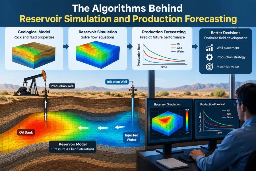

A reservoir engineer may be asked a deceptively simple question: if a new well is drilled next year, how much oil, gas, and water will it produce? The answer affects platform capacity, pipeline sizing, capital decisions, reserves reporting, and the day-to-day plan for operating a field.
Yet nobody can see the reservoir directly. Engineers work from scattered well logs, core samples, pressure measurements, seismic interpretation, fluid tests, and production history. They must turn those partial observations into a defensible view of a rock volume that may extend for many kilometres underground.
Reservoir simulation is the computational framework used to make that view dynamic. It calculates how fluids move through porous rock as wells produce or inject fluids, then converts assumptions about geology and operations into production forecasts.
The algorithms are not crystal balls. They are structured ways to apply physics, data, and uncertainty. Understanding what they calculate—and where they can mislead—makes forecast discussions far more useful for students and working professionals alike.
🗺️ The Reservoir as a Hidden Flow System
A petroleum reservoir is not an underground lake. It is a connected volume of rock containing tiny pore spaces, often filled with combinations of oil, gas, and water. Fluid can move only through connected pores and fractures, and the ease of movement varies sharply from one location to another.
A simulator represents this hidden system through variables such as pressure, fluid saturation, permeability, porosity, depth, and temperature. Its central task is to estimate how those variables change through time when wells alter the reservoir’s pressure and fluid balance.
🧱 Why Engineers Divide Rock into Grid Cells
Because a reservoir is too complex to solve as one continuous object, simulation models divide it into many grid cells. Each cell carries average rock and fluid properties, while connections between neighboring cells describe possible pathways for flow.
This is similar to representing a landscape with pixels. Small cells can describe faults, channels, and wellbore neighborhoods more clearly, but they also create a much larger numerical problem. The grid must be detailed enough for the decisions at hand, not simply as fine as available computing power permits.
⚖️ The Conservation Laws at the Core
Every conventional reservoir simulator starts with conservation of mass. For each fluid phase—water, oil, and gas—the change in mass stored in a cell must equal mass flowing in, minus mass flowing out, plus any wells or sources.
The model also needs a flow relationship, usually Darcy’s law. In simplified form, it says fluid flow increases with pressure difference and rock permeability, and decreases with fluid viscosity and travel resistance. These relationships allow the simulator to translate pressure gradients into phase flow rates.
💧 Why Multiphase Flow Changes Everything
Oil, water, and gas do not move independently through the same pore channels. When water saturation rises, for example, it may block routes previously available to oil. This interaction is represented by relative permeability, which describes each phase’s effective ability to flow at a given saturation.
Capillary pressure adds another effect: different fluids can sustain different pressures in small pores because of interfacial forces. These functions are often measured on core samples or inferred from analog data, but scale and sample representativeness remain major uncertainties.
🧪 Fluid Models Describe Changing Hydrocarbons
Reservoir fluids can change substantially as pressure falls. Gas may come out of solution, oil volume can shrink, and a gas condensate system may form liquid near the wellbore. A production forecast therefore needs more than a single oil density and viscosity.
Black-oil models use engineering tables to represent common oil, water, and gas behavior efficiently. More detailed compositional models track hydrocarbon components and phases explicitly. They are especially useful when phase behavior, gas injection, volatile oils, or condensate dropout materially influence recovery.
🧮 From Differential Equations to Cell Balances
Flow equations are continuous in space and time, but computers solve finite sets of equations. Spatial discretization replaces the reservoir with cell balances, while time discretization advances the solution from one reporting point to the next.
For a cell, the simulator calculates stored fluid and all fluxes through its faces. Repeating this across the grid produces a linked system: a pressure change in one area can eventually alter flow behavior elsewhere, particularly in well-connected formations.
⏱️ Time Steps Are a Numerical Decision
The simulator does not usually jump directly from today to next year. It moves in time steps, which may be short around a well startup, a pressure transient, or a control change, and longer during quieter periods.
Large time steps reduce run time but can miss sharp saturation or pressure changes. Very small steps improve resolution but may add little decision value. Adaptive time stepping lets the solver reduce the step after difficulty and expand it when the reservoir response is smooth.
🔢 Why Reservoir Equations Are Nonlinear
Reservoir flow is nonlinear because properties depend on the unknowns being solved. Pressure changes density and fluid volume; saturation changes relative permeability; gas appearance changes phase mobility; and well controls may switch during a calculation.
That means the simulator repeatedly guesses a solution, evaluates the mismatch in each equation, and updates the guess. Newton-type methods are widely used because they can converge rapidly near a solution, though they can struggle when the initial estimate or time step is unsuitable.
🧩 Linear Solvers Do the Heavy Computational Work
After a nonlinear iteration is linearized, the program must solve a very large system of simultaneous equations. Modern reservoir models may contain hundreds of thousands or millions of active cells, so this operation dominates computational cost.
Iterative solvers exploit the sparse structure of the matrix: each cell interacts directly with only a limited number of neighbors. Preconditioners reshape the numerical problem so the iterative method reaches an acceptable answer in fewer steps. This is numerical engineering, not a minor software detail.
🧭 Fully Implicit and Explicit Solution Choices
A fully implicit formulation solves pressure and saturations together at the new time level. It is generally robust for difficult multiphase problems and permits larger time steps, but each step is computationally expensive.
Explicit or sequential approaches can be faster in favorable conditions, often solving pressure and transport separately. Their drawback is tighter stability limits or reduced robustness when flow conditions change rapidly. The best approach depends on physics, grid size, required accuracy, and workflow speed.
📐 Geometry, Faults, and Transmissibility
Cells exchange fluid through a quantity commonly called transmissibility. It combines face area, distance, rock permeability, and fluid mobility to describe how readily fluid crosses from one cell to another.
Faults require particular care. A mapped fault may be sealing, partially sealing, or transmissive; its behavior can vary along strike. Assigning a single extreme assumption without pressure or production support can create forecasts that look precise while resting on a weak geological interpretation.
🕳️ Wells Need Their Own Flow Model
A well is not simply a cell with a negative flow rate. The connection between wellbore and grid block must account for completion interval, local permeability, skin, well radius, and pressure drawdown. This relationship is often expressed through a well index.
For horizontal and fractured wells, near-well representation becomes especially influential. A coarse grid may smear the pressure response, while simplified completion assumptions can distort predicted productivity and breakthrough timing.
🎛️ Controls Turn Physics into an Operating Plan
Wells operate under constraints. A producer might be held at a target liquid rate until its bottom-hole pressure reaches a limit, then switch to pressure control. An injector may be constrained by maximum rate, pressure, or available injection volume.
These rules matter because a forecast is a simulation of a development plan, not merely reservoir depletion. Facility limits, water handling capacity, gas sales constraints, and downtime assumptions can all determine field output even when reservoir deliverability is higher.
📈 Production Forecasting Starts with a Base Case
A base case states a coherent set of geological, fluid, well, and operating assumptions. It may include existing production, planned wells, injection strategy, workovers, and expected constraints. The simulator then generates rates, cumulative volumes, pressure, water cut, gas-oil ratio, and saturation maps.
A forecast should be read as conditional: “given these inputs and controls, this is the modeled response.” It is not a promise that future production will follow the curve exactly.
🔄 History Matching Connects Model and Reality
History matching adjusts uncertain model inputs so simulated behavior reasonably reproduces observed field history. Common match targets include oil, gas, and water rates; flowing and static pressures; water breakthrough; gas-oil ratio; and pressure interference between wells.
A visually close rate match alone is not sufficient. An unrealistic model can compensate for a wrong permeability distribution with an altered aquifer, well skin, or relative permeability curve. Strong history matching uses multiple independent observations to reduce these compensating errors.
🧠 Calibration Is Not Proof of Uniqueness
Many different combinations of uncertain inputs can match the same production history. This issue, known as non-uniqueness, is central to reservoir modeling. A match may describe past observations well while implying very different future behavior.
Engineers manage this by preserving geological plausibility, honoring measured data, and testing alternative model realizations. The goal is not to find one supposedly perfect model; it is to identify a credible range of models that answer the decision question.
🌊 Aquifers Can Sustain or Complicate Production
An aquifer is a connected water-bearing volume that can provide pressure support as hydrocarbons are produced. In a model, it may be represented explicitly with water-filled grid cells or through a simplified analytical aquifer relationship.
Strong support can maintain pressure and improve oil displacement, but it can also accelerate water production. Treating an uncertain aquifer as a fixed background detail is risky because it affects pressure decline, recovery, water handling, and the value of injection plans.
💉 Injection Forecasts Depend on Sweep, Not Just Volume
Waterflooding and gas injection aim to move hydrocarbons toward producers or maintain pressure. Injected volume alone does not guarantee recovery. The displacement must contact oil-bearing rock and avoid bypassing it through high-permeability streaks, fractures, or unfavorable mobility conditions.
Simulation helps compare patterns, injection rates, and well placement by tracking saturation movement. It can identify an early breakthrough risk, but predictions remain sensitive to heterogeneity that is often only partly constrained between wells.
🧊 Enhanced Recovery Requires Extra Physics
Thermal recovery, polymer flooding, surfactant processes, miscible gas injection, and low-salinity concepts can require specialized models. Temperature, component transport, adsorption, chemical reactions, viscosity changes, and interfacial behavior may be relevant.
More physics is valuable only when it is supported by the decision and available data. A highly complex model with poorly known input functions can create false confidence. Laboratory work, pilot results, and sensitivity analysis should guide the level of detail.
📊 Decline Curves and Simulation Answer Different Questions
Decline-curve analysis extrapolates production trends from historical data. It can be fast, transparent, and very useful for mature wells with stable operating conditions. Reservoir simulation represents mechanisms and can test changes in wells, injection, constraints, and field development.
| Method | Best use | Main limitation |
|---|---|---|
| Decline analysis | Trend-based estimates for established production | Weak for major operational or reservoir changes |
| Material balance | Volumetric and pressure-support understanding | Limited spatial detail |
| Reservoir simulation | Well placement and scenario-based development planning | Requires many uncertain inputs and careful calibration |
These methods are complementary. A mismatch between them is often a useful diagnostic question, not an automatic reason to discard one result.
🎲 Uncertainty Must Be Designed into Forecasts
Key uncertainties may include connected volume, fault transmissibility, permeability distribution, relative permeability, aquifer strength, well productivity, uptime, and future operating constraints. A single deterministic forecast hides the impact of those choices.
Scenario analysis changes a few coherent assumptions to create low, central, and high cases. Probabilistic workflows sample defined uncertainty distributions across many realizations. Neither method removes uncertainty; each makes it visible so decisions can account for downside and upside.
🧷 Sensitivity Analysis Finds What Actually Matters
Not every uncertain parameter deserves the same effort. Sensitivity analysis varies inputs and observes the response in a selected metric, such as cumulative oil, plateau duration, water rate, or net injection requirement.
A practical workflow first screens broad uncertainties, then focuses detailed studies on parameters that materially change the decision. If forecast value is insensitive to a parameter, refining it may have little benefit. If a fault seal assumption controls the result, new pressure data or surveillance may be valuable.
🤖 Surrogate Models Can Speed Up Decisions
Full-physics simulation can be too slow for optimization across thousands of possible well locations or control schedules. A surrogate model, sometimes called a proxy, learns an approximation from a set of simulator runs and evaluates new cases quickly.
Machine-learning methods can support this task, but they inherit the assumptions and coverage of their training simulations. A proxy should be checked against withheld full-model cases, particularly near operating limits or in regions where the model is extrapolating.
🧬 Data Assimilation Updates Forecasts Over Time
A reservoir model should evolve as production and surveillance data arrive. Data assimilation methods update model parameters or model ensembles using new pressure, rate, tracer, seismic, or saturation information while accounting for uncertainty.
The practical principle is straightforward: do not treat the original forecast as permanent. Reforecast after material changes in field behavior, new well results, revised fluid data, or operational constraints. A living model supports better decisions than an archived one.
🔍 Quality Control Begins Before the First Run
Simulation errors are often caused by input problems rather than advanced numerical failures. Unit inconsistencies, wrong depth references, unconnected grid cells, negative pore volumes, incorrect completion intervals, and implausible fluid tables can all corrupt results.
- Check original fluids in place against volumetric estimates.
- Confirm well rates, signs, dates, and allocation conventions.
- Inspect maps of porosity, permeability, saturation, and net-to-gross.
- Test that initial pressure and fluid contacts are physically consistent.
- Review material balance and cumulative injection-production volumes.
These checks are basic, but they prevent polished-looking forecasts from being built on flawed foundations.
⚠️ Common Ways Forecasts Become Misleading
A common mistake is over-refining the grid around wells while leaving large-scale connectivity poorly understood. Another is matching every historical wiggle in production by changing unconstrained parameters, effectively fitting noise or operational artifacts rather than reservoir behavior.
Forecasts also become misleading when assumptions are buried in model files instead of communicated clearly. A decision maker needs to know whether a result depends on uninterrupted uptime, injector performance, a particular facility expansion, or an uncertain geological connection.
🗣️ Good Communication Makes Models Decision-Ready
A technically sound model can still fail to support a decision if its output is unreadable. Start with the decision, the forecast range, the major drivers, and the conditions that would change the recommendation. Then provide technical detail appropriate to the audience.
Useful visuals include production profiles with constraints shown, cumulative distributions, pressure trends, maps of remaining oil, and comparisons of alternative development concepts. Avoid presenting a single smooth curve without its assumptions and uncertainty context.
🛠️ A Practical Workflow for New Practitioners
Students and early-career engineers often benefit from a disciplined sequence rather than starting with software menus. The model should grow from a clear question, not from a desire to use every available feature.
- Define the decision and forecast horizon.
- Assemble and quality-check geological, petrophysical, PVT, pressure, and production data.
- Build an initial static model and calculate volumes.
- Select fluid and flow physics appropriate to the reservoir.
- Construct wells, controls, and historical operations.
- History match against several relevant observations.
- Run sensitivities and alternative development cases.
- Document assumptions, limitations, and surveillance needed to reduce uncertainty.
🎓 The Core Principle Behind Useful Forecasts
The strongest reservoir forecast is not the one with the most cells, the longest input deck, or the smoothest match plot. It is the one that uses appropriate physics, honors available evidence, exposes material uncertainty, and addresses a real operating or investment decision.
Algorithms provide the discipline to calculate thousands of interacting flow effects consistently. Engineering judgment decides which assumptions are credible, which uncertainties matter, and when new field data should change the plan.
Reservoir simulation is most valuable when it is treated as a transparent, continuously tested decision tool—not as a machine that produces certainty from incomplete subsurface data. 🛢️📈🔬